# Set up to be able to use python for symbolic math help.
from sympy import *
from sympy.assumptions.assume import global_assumptions
from IPython.display import display, Math, Latex # Latex printing in notebook

l, t, m1, m2, g = symbols("l t m1 m2 g", real=True, positive=True)
p1x = Function("p1x", real=True)(t)
theta = Function("theta", real=True)(t)
global_assumptions.add(Q.real(theta.diff(t)))
global_assumptions.add(Q.real(p1x.diff(t)))
thetaDot = theta.diff(t, real=True)

Suppose we have a mass attached to a cart depicted in following diagram:

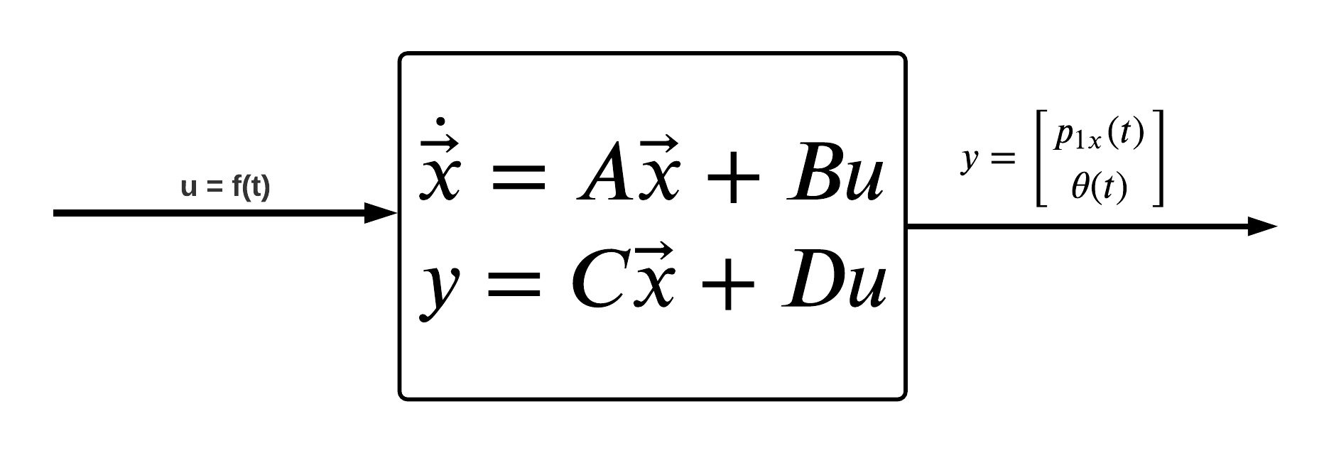
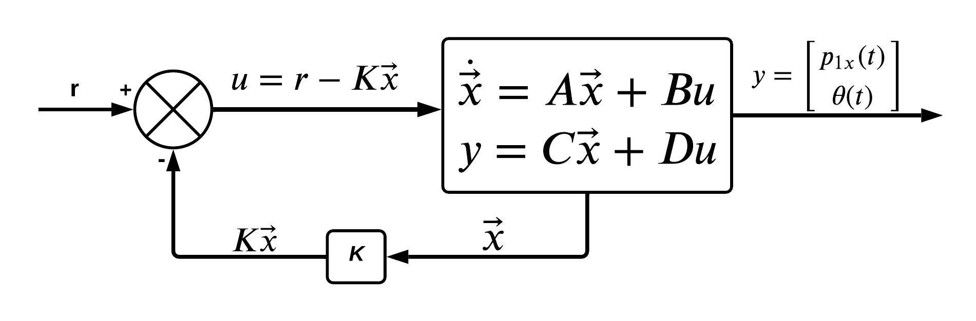
We wish to control the system such that the $m2$ mass will remain in the upright and vertical position. To keep the $m2$ mass in the upright vertical position i.e. keeping $\theta = 0$, we will be applying some force $f(t)$ on the $m1$ mass in the horizontal direction. To determine the magnitude and direction of the force needed to keep the $m2$ mass balanced, we will be using a full state feedback controller.

In order create a state feedback controller to balance our $m2$ mass, we must first come up with a mathematical model of our system, a.k.a the equations of motion (EOM). For this exercise, we opted to use Lagrangian mechanics to derive our EOM.

Note: We could have derived the EOMs using Newton's 2nd law, but found the math to be much more simple when using the Lagrangian.

In order to use the Lagrangian, we must fully describe the kinetic and potential energies of the system. This is more easily achieved if we add a few position vectors to our system diagram:

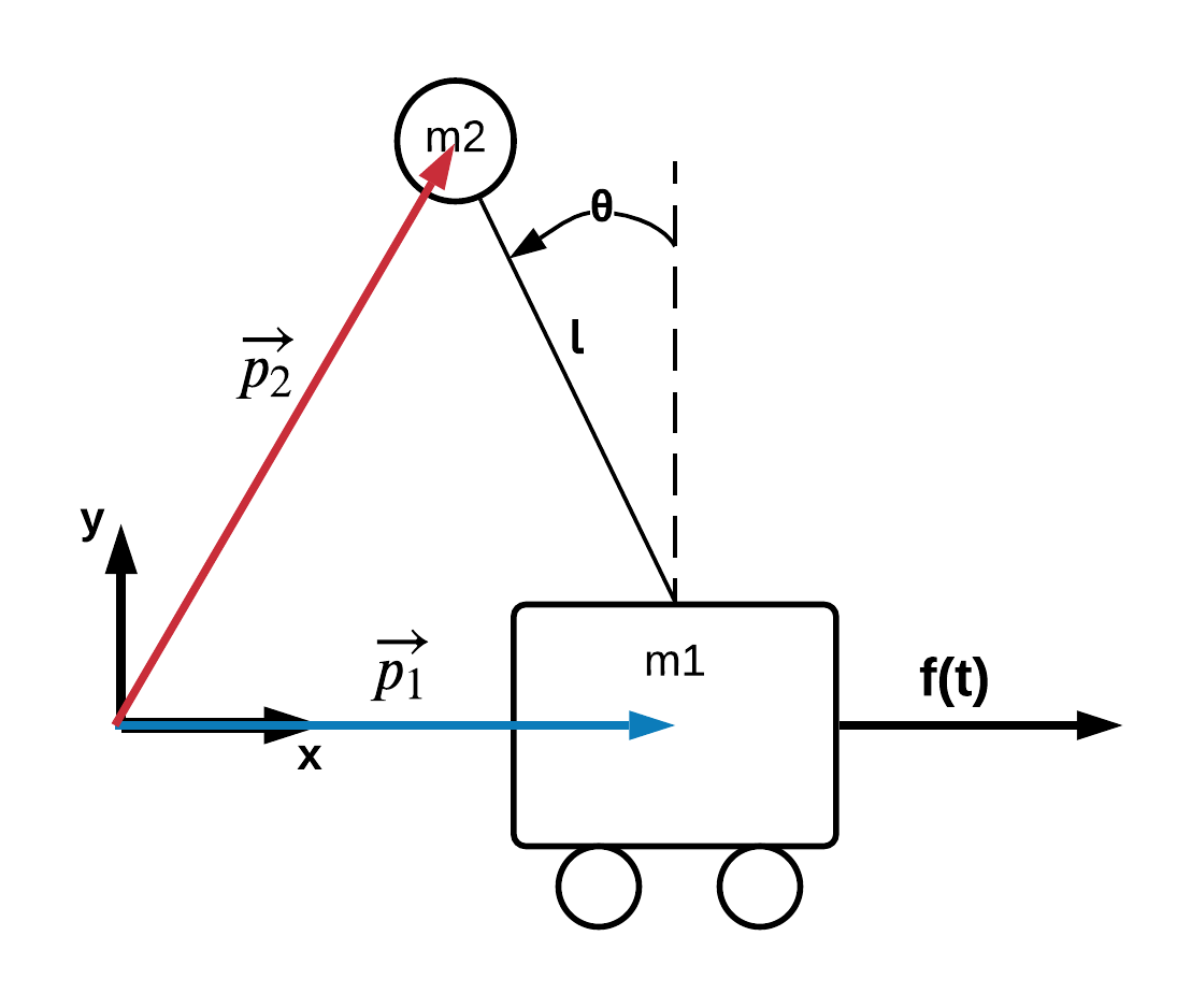
With the vectors $\vec{p_1}$ and $\vec{p_2}$ we can now describe the kinetic and potential energies as follows:

$$ KE = \frac{1}{2} m_1 \lvert \dot {\vec p_1} \rvert ^2 + \frac{1}{2} m_2 \lvert \dot {\vec p_2} \rvert ^2 \\ \tag{1} \label{keNotUseful} $$$$ PE = m_2 g l cos(\theta) \\ \tag{2} \label{pe} $$

While the equation listed at $\eqref{keNotUseful}$ is very true, it is not very helpful. When we go to implement, we will not be able to directly measure or approximate $\vec p_2$ or $\dot{\vec p_2}$. We can however solve for $\vec p_2$ and $\dot{\vec p_2}$ in terms of other variables we can measure and approximate such as $\vec p_1$ and $\dot {\vec p_1}$.

Note: In the controls world, we typically call the variables that we can measure and/or calculate in real-time 'states'.

Consider our system but while only looking at the following vectors:

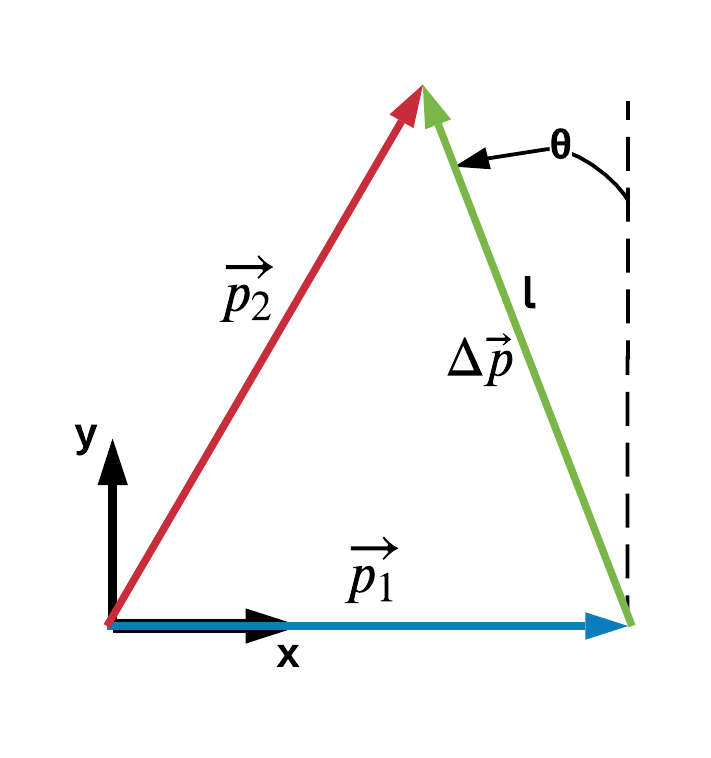
We can say that $$ \vec{p_2} = \vec{p_1} + \Delta \vec{p} \\ \tag{3} $$

Using the vector diagram, we can substitute useful relationships for $\vec{p_1}$ and $\Delta \vec{p}$ to represent $\vec{p_2}$ in terms of states that we can measure or approximate.

p1Vec = Matrix([p1x, 
                0], real=True)
display(Math(r"\vec{p_1} = {}"), p1Vec)

$\displaystyle \vec{p_1} = {}$

$\displaystyle \left[\begin{matrix}\operatorname{p1x}{\left(t \right)}\\0\end{matrix}\right]$

deltaPVec = Matrix([-l*sin(theta),
                   l*cos(theta)], real=True)
display(Math(r"\Delta \vec{p} ="), deltaPVec)

$\displaystyle \Delta \vec{p} =$

$\displaystyle \left[\begin{matrix}- l \sin{\left(\theta{\left(t \right)} \right)}\\l \cos{\left(\theta{\left(t \right)} \right)}\end{matrix}\right]$

p2Vec = p1Vec + deltaPVec
display(Math(r"\vec{p_2} = \vec{p_1} + \Delta \vec{p} = "), p2Vec)

$\displaystyle \vec{p_2} = \vec{p_1} + \Delta \vec{p} = $

$\displaystyle \left[\begin{matrix}- l \sin{\left(\theta{\left(t \right)} \right)} + \operatorname{p1x}{\left(t \right)}\\l \cos{\left(\theta{\left(t \right)} \right)}\end{matrix}\right]$

We can now use these relationships for $\vec{p_1}$ and $\vec{p_2}$ to determine $\lvert \dot{\vec{p_1}} \rvert$ and $\lvert \dot{\vec{p_2}} \rvert$ in terms of known constants and measurable values.

p1VecDotNorm = p1Vec.diff(t).norm()
display(Math(r"\lvert \dot{\vec{p_1}} \rvert = "),p1VecDotNorm)

$\displaystyle \lvert \dot{\vec{p_1}} \rvert = $

$\displaystyle \left|{\frac{d}{d t} \operatorname{p1x}{\left(t \right)}}\right|$

p2VecDotNorm = simplify(refine(p2Vec.diff(t).norm()))
display(Math(r"\lvert \dot{\vec{p_2}} \rvert = "), p2VecDotNorm)

$\displaystyle \lvert \dot{\vec{p_2}} \rvert = $

$\displaystyle \sqrt{l^{2} \left(\frac{d}{d t} \theta{\left(t \right)}\right)^{2} - 2 l \cos{\left(\theta{\left(t \right)} \right)} \frac{d}{d t} \operatorname{p1x}{\left(t \right)} \frac{d}{d t} \theta{\left(t \right)} + \left(\frac{d}{d t} \operatorname{p1x}{\left(t \right)}\right)^{2}}$

Now that we have $\vec{p_1}, \lvert \dot{\vec{p_1}} \rvert, \vec{p_2}, \lvert \dot{\vec{p_2}} \rvert$ all in terms of useful states, we can express our Lagrangian entirely in terms of useful states.

ke = 1/2*m1*p1VecDotNorm**2  + 1/2*m2*p2VecDotNorm**2
pe = m2*g*l*cos(theta)
L = simplify(refine(ke - pe))
display(Math(r"L ="),L)

$\displaystyle L =$

$\displaystyle - g l m_{2} \cos{\left(\theta{\left(t \right)} \right)} + 0.5 m_{1} \left(\frac{d}{d t} \operatorname{p1x}{\left(t \right)}\right)^{2} + 0.5 m_{2} \left(l^{2} \left(\frac{d}{d t} \theta{\left(t \right)}\right)^{2} - 2 l \cos{\left(\theta{\left(t \right)} \right)} \frac{d}{d t} \operatorname{p1x}{\left(t \right)} \frac{d}{d t} \theta{\left(t \right)} + \left(\frac{d}{d t} \operatorname{p1x}{\left(t \right)}\right)^{2}\right)$

Now that we have our Lagrangian, we can get our EOM by evaluating the following:

$$ \frac{d}{dt}\left\lgroup \frac{\partial L}{\partial \dot x}\right\rgroup-\frac{\partial L}{\partial x}=f(t) \\ \tag{4} \label{eom1} $$$$ \frac{d}{dt}\left\lgroup \frac{\partial L}{\partial \dot \theta}\right\rgroup-\frac{\partial L}{\partial \theta}=0 \\ \tag{5} \label{eom2} $$

Note: If you need a refresher of Lagrangian mechanics, we found the following videos to be useful:

• https://youtu.be/4uJaKJASKnY
• https://youtu.be/uFnTRJ2be7I

eom1, eom2 = euler_equations(L, [p1x, theta], t)
f = Function("f")
eom1 = eom1.subs(0, -f(t))
display(simplify(eom1))

$\displaystyle f{\left(t \right)} = 1.0 m_{1} \frac{d^{2}}{d t^{2}} \operatorname{p1x}{\left(t \right)} + m_{2} \left(l \sin{\left(\theta{\left(t \right)} \right)} \left(\frac{d}{d t} \theta{\left(t \right)}\right)^{2} - l \cos{\left(\theta{\left(t \right)} \right)} \frac{d^{2}}{d t^{2}} \theta{\left(t \right)} + \frac{d^{2}}{d t^{2}} \operatorname{p1x}{\left(t \right)}\right)$

$$ = \frac{d}{dt}\left\lgroup \frac{\partial L}{\partial \dot x}\right\rgroup-\frac{\partial L}{\partial x}=f(t) $$

display(simplify(eom2))

$\displaystyle l m_{2} \left(g \sin{\left(\theta{\left(t \right)} \right)} - l \frac{d^{2}}{d t^{2}} \theta{\left(t \right)} + \cos{\left(\theta{\left(t \right)} \right)} \frac{d^{2}}{d t^{2}} \operatorname{p1x}{\left(t \right)}\right) = 0$

$$ = \frac{d}{dt}\left\lgroup \frac{\partial L}{\partial \dot \theta}\right\rgroup-\frac{\partial L}{\partial \theta}=0 $$

Now that we have our EOM, we want to represent our system in a way that makes it easy to control. Since we have decided to use a full-state feedback controller, we want to represent our system in the following form:

$$ \dot{\vec{x}}= A \vec x + Bu \\ \tag{6} \label{stateEq} $$$$ y = C \vec x + Du \\ \tag{7} \label{outputEq} $$

Note: If the state equation $\eqref{stateEq}$ or the output equation $\eqref{outputEq}$ seem unfamiliar, then we highly suggest watching the following video:

• https://youtu.be/hpeKrMG-WP0

In order to simplify our lives and be able to express A in terms of only constants, we decide to apply the following simplifications:

Note: The following approximations are justified for $-5 ^{\circ} \leq \theta \leq 5 ^{\circ} $: $$ cos\theta \approxeq1 \\ sin\theta\approxeq\theta \\ $$

Note: The following approximation is valid since $\dot\theta$ will be relatively small: $$ \dot\theta^2\approxeq 0 $$

linearizations = [
    (sin(theta), theta),
    (cos(theta), 1),
    (thetaDot**2, 0)
]
eom1 = eom1.subs(linearizations)
eom1 = simplify(eom1)

eom2 = eom2.subs(linearizations)
eom2 = simplify(eom2)

print("eom1 after linearization:")
display(eom1)

eom1 after linearization:

$\displaystyle f{\left(t \right)} = 1.0 m_{1} \frac{d^{2}}{d t^{2}} \operatorname{p1x}{\left(t \right)} - m_{2} \left(l \frac{d^{2}}{d t^{2}} \theta{\left(t \right)} - \frac{d^{2}}{d t^{2}} \operatorname{p1x}{\left(t \right)}\right)$

print("eom2 after linearization:")
display(eom2)

eom2 after linearization:

$\displaystyle l m_{2} \left(g \theta{\left(t \right)} - l \frac{d^{2}}{d t^{2}} \theta{\left(t \right)} + \frac{d^{2}}{d t^{2}} \operatorname{p1x}{\left(t \right)}\right) = 0$

Now that we have linearized our EOM, let us explicitly say what our states are: $$ \vec x = \left [ \begin{matrix} p_{1x} \\ \dot p_{1x} \\ \theta \\ \dot\theta \\ \end{matrix} \right ] \implies \dot{\vec x} = \left [ \begin{matrix} \dot{p_{1x}} \\ \ddot{p_{1x}} \\ \dot{\theta} \\ \ddot{\theta}\\ \end{matrix} \right ] $$

We will now solve our equations of motion for $\ddot{\theta}$ and $\ddot{p_{1x}}$. This gets us one step closer to be able to represent our system in the following form: $$ \dot{\vec{x}}= A \vec x + Bu \\ y = C \vec x + Du $$

# Defining symbolic variables
thetaDotDot = thetaDot.diff(t, real=True)
p1xDotDot = p1x.diff(t, real=True).diff(t, real=True)

# Solving for thetaDotDot and p1xDotDot
solution = solve([eom1, eom2], [thetaDotDot, p1xDotDot])

# Getting the solutions of thetaDotDot and p1XDotDot out 
# of a dictionary
thetaDotDot = simplify(solution[thetaDotDot])
p1xDotDot = simplify(solution[p1xDotDot])

display(Math(r"\ddot{\theta} ="), thetaDotDot)

$\displaystyle \ddot{\theta} =$

$\displaystyle \frac{g m_{1} \theta{\left(t \right)} + g m_{2} \theta{\left(t \right)} + f{\left(t \right)}}{l m_{1}}$

display(Math(r"\ddot{p_{1x}} = "), p1xDotDot)

$\displaystyle \ddot{p_{1x}} = $

$\displaystyle \frac{g m_{2} \theta{\left(t \right)} + f{\left(t \right)}}{m_{1}}$

Now that we have expressions for $\ddot{\theta}$ and $\ddot{p_{1x}}$ in terms of our states, we are ready to represent the system in terms of the state equation and the output equation.

p1xDot = p1x.diff(t)
x = [p1x, p1xDot, theta, thetaDot]
xDot = [p1xDot, p1xDotDot, thetaDot, thetaDotDot]

# type conversions are needed for the linear_eq_to_matrix function call to work
typeConversions = [
    (p1xDot, Symbol("p1xDot")),
    (thetaDot, Symbol("thetaDot")),
    (p1x, Symbol("p1x")),
    (theta, Symbol("theta")),
    (f(t), Symbol("f(t)"))
]

for i in range(len(xDot)):
    xDot[i] = xDot[i].subs(typeConversions)
    x[i] = x[i].subs(typeConversions)

# Gives the variables in the following form 
# xDot = A*x - B*u
APlant, B = linear_eq_to_matrix(xDot, x)

# Changing to the form
# xDot = A*x + B*u
B = -1*B

# Getting f(t) out of the B matrix
B = B.subs(Symbol("f(t)"), 1)

display(Math(r"A ="), APlant)

$\displaystyle A =$

$\displaystyle \left[\begin{matrix}0 & 1 & 0 & 0\\0 & 0 & \frac{g m_{2}}{m_{1}} & 0\\0 & 0 & 0 & 1\\0 & 0 & \frac{g m_{1} + g m_{2}}{l m_{1}} & 0\end{matrix}\right]$

display(Math(r"B ="), B)

$\displaystyle B =$

$\displaystyle \left[\begin{matrix}0\\\frac{1}{m_{1}}\\0\\\frac{1}{l m_{1}}\end{matrix}\right]$

C = Matrix([[1, 0, 0, 0],
            [0, 0, 0, 0],
            [0, 0, 1, 0],
            [0, 0, 0, 0]])

display(Math(r"C ="), C)

$\displaystyle C =$

$\displaystyle \left[\begin{matrix}1 & 0 & 0 & 0\\0 & 0 & 0 & 0\\0 & 0 & 1 & 0\\0 & 0 & 0 & 0\end{matrix}\right]$

D = Matrix([0,
            0,
            0,
            0])
display(Math(r"D = "), D)

$\displaystyle D = $

$\displaystyle \left[\begin{matrix}0\\0\\0\\0\end{matrix}\right]$

Now is a good time to substitue some actual values for our constants and do some sanity checks. We want to plot the poles of the system and check that at least one is in the right half plane.

from control.matlab import *
import matplotlib.pyplot as plt
import numpy as np
from math import pi

measuredValues = [
    (g, 9.81),
    (m1, 1.0),
    (m2, 2.0),
    (l, 1.0)
]
APlant = APlant.subs(measuredValues)
B = B.subs(measuredValues)

sys = StateSpace(APlant, B, C, D)
fig0 = plt.figure()
p0 = pzmap(sys)

As seen in the figure above a pole is in the right half plane, meaning the system is inherently unstable. This makes sense, since the pendulum would not remain in the upright vertical position if we were not actively trying to balance the pendulum.

The objective of our statespace controller should be to move the pole in the right half plane to the left half.

In general, state feeback controllers take a plant as illustrated in the figure below:

The state is 'fed back' to the input while applying a individual gains K to each state variable. Applying these gains and feedback ultimately is what moves the poles of the overall system. A figure illustrating the state feedback controller being applied to the plant can be found below:

One question you may be asking yourself is how do we determine each of the gains for K such that the system's poles get moved to the left hand plane?

Probably the best way to show how we determine the gains for K is through a little derivation. We will prove:

1. The state equation and the output equation can be represented as a transfer function.
2. The eigenvalues of the A matrix in the state equation represent the poles of our system.

Let's begin with proving the state equation $\dot{\vec{x}} = A \vec x + Bu$ and the output equation $y = C\vec x + Du$ can be represented as a transfer function.

First let's take the Laplace transfrom of both the state equation and the output equation:

$$ sX(s) = A X(s) + B U(s) \\ Y(s) = C X(s) + D U(s) $$

Now let's isolate for $X(s)$ in the state equation:

$$ s X(s) - A X(s) = B U(s) \\ X(s)(sI - A) = B U(s) \\ X(s) = (sI - A)^{-1}B U(s) $$

In many cases (including our inverted pendulum) we choose our $D = \mathbf{0}$. Let's express this simplification in our output equation:

$$ Y(s) = CX(s) $$

Let's substitute $X(s)$ for the expression we derived in the state equation:

$$ Y(s) = C(sI - A)^{-1}B U(s) $$

Since $U(s)$ is a 1x1, we can solve for the transfer function by dividing $U(s)$ to both sides of the equation:

$$ \frac{Y(s)}{U(s)} = G(s) \\ = C(sI - A)^{-1}B \\ $$$$ = C \frac{\mathrm{adj}(sI - A)}{\det(sI - A)} B \label{transferFunction} \tag{8} $$

As seen in equation $\eqref{transferFunction}$ the poles for the system can be determined by setting the $\det(sI -A) = 0$. As it turns out, solving for the values of $s$ that cause the denominator to be zero is the same as if we had determined the eigenvalues for A.

An aside: The relationship between the poles of our system and the eigenvalues of the A matrix become apparent if we look at the definition of an eigenvector and try to solve for the eigenvalues: $$ A\vec{v} = \lambda \vec{v} \\ \lambda \vec{v} - A\vec{v} = \mathbf{0} \\ =(\lambda I - A)\vec{v} = \mathbf{0} $$

We would then solve for the eigenvalues by finding the $\det(\lambda I - A) = 0$. Notice that the $\det(\lambda I -A) = 0$ would be identical to the denominator of equation $\eqref{transferFunction}$ if we substitute $\lambda$ for $s$.

If you are uncertain why we took the $\det(\lambda I - A)$ and set it equal to $\mathbf{0}$ then consider watching the following video:

• https://youtu.be/rfm0wQObxjk

Okay, we have proven that the state space representation our system can be converted into a transfer function and the poles of that transfer function are the eigenvalues of our $A$ matrix. Lets now look at applying feedback and how that affects the $A$ matrix of the closed-loop system. Looking back at our closed-loop model:

Let's now substitute $u=r-K\vec x$ into our state equation:

$$ \dot{\vec x} = A \vec x + B (r - K\vec x) $$

Let's see if we can expand and factor out our $\vec x$.

$$ \dot{\vec x} = A \vec x + Br - BK\vec x \\ = A \vec x - BK\vec x + Br $$$$ = (A - BK)\vec x + Br \label{aClosedLoop} \tag{9} $$

Equation $\eqref{aClosedLoop}$ should look very familiar. If we substitute $(A-BK)$ for $A_{closed loop}$, we will see equation $\eqref{aClosedLoop}$ is in the exact same form as our original state equation:

$$ \dot{\vec{x}} = A_{closed loop} \vec x + Br $$

We can now say that the eigenvalues for the overall system are at the eigenvalues of $A_{closed loop}$. We can solve for our $K$ matrix by setting the characteristic equation of $A_{closed loop}$ to our desired characteristic equation: $$ \det(A_{closed loop}) = \mathrm{desiredCharEq} $$

k1, k2, k3, k4 = symbols(["k1", "k2", "k3", "k4"])
s = Symbol("s")
K = Matrix([[k1, k2, k3, k4]])
AClosedLoop = APlant - B*K
charEq = det(s*eye(4) - AClosedLoop)

To find our gain values we must choose some performance criteria for the transient response, namely the maximum settling time and percent overshoot. This produces a 2nd-order characteristic polynomial to which we add two more terms to make the overall 'desired' polynomial a 4th-order. The added terms simply place then two remaining roots (poles) at 5x the distance of the other two on the real axis. We can then set this equal to our actual characteristic equatioin and solve for our gains by matching like-terms: $$ \omega_n=\frac{4}{\zeta T_s} \\ \zeta=\frac{-\ln(\frac{\%OS}{100})}{\sqrt{\pi^2+\ln^2(\frac{\%OS}{100})}} \\ \mathrm{desiredCharEq} = (s^2+2\zeta\omega_ns+\omega_n^2)(s+5\zeta\omega_n)^2 = \det(A_{closed loop}) $$

# Requirements we are trying to achieve
os = 0.10 # Overshoot
TSetSeconds = 2.0 # Settling time

zet = -ln(os)/sqrt(pi**2 + ln(os)**2)
wn = 4/(zet*TSetSeconds)

desiredCharEq = (s + zet*wn + I*wn*sqrt(1 - zet**2)) * (s + zet*wn - I*wn*sqrt(1 - zet**2)) * (s + 5*wn*zet)**2

gains = solve(Eq(charEq, desiredCharEq), K)
gainsSub = [
    (k1, gains[k1]),
    (k2, gains[k2]),
    (k3, gains[k3]),
    (k4, gains[k4])
]

Now that we have solved for the gains that move the poles to the desired locations. We should plot where the poles are and confirm they are at their desired locations.

AClosedLoop = AClosedLoop.subs(gainsSub)

initialStates = [0, # p1x (m)
                 0, # p1xdot (m/s)
                 5 * pi / 180, # theta (rad)
                 0] # thetadot (rad/sec) 
                        
sys = StateSpace(AClosedLoop, B, C, D)
fig1 = plt.figure()
p1 = pzmap(sys)

Okay, we have reason to believe the system is now stable. Let's see what happens to $\theta$ when we give it an intial displacement of $5^\circ$.

fig2 = plt.figure()
dt = 0.01
T = np.arange(0, 3, dt)
y, t = initial(sys, T, initialStates)
thetaDeg = y[:, 2] * 180/pi
p1 = plt.plot(t, thetaDeg)
plt.title("$\Theta$ vs t")
plt.ylabel("$\Theta$ ($\degree$)")
plt.ylim([-4, 5.5])
plt.xlabel("t (sec)")
plt.grid("on")

As seen in the plot above, $\theta$ will approch $0$ as $t \to \infty$. This gives us reason to believe our control theory is correct and we are ready to begin implementation.